在上一章中，我们学习了如何创建机器学习和深度学习模型，以及如何在 Azure Databricks 中的分布式训练期间加载数据集。找到正确的机器学习算法来使用机器学习解决问题是一回事，但找到最佳超参数是另一个同样或更复杂的任务。在本章中，我们将重点关注使用 MLflow 作为模型存储库的模型调优、部署和控制。我们还将使用 Hyperopt 为我们的模型搜索最佳超参数集。我们将使用使用 scikit-learn Python 库制作的深度学习模型来实现这些库的使用。

更具体地说，我们将学习如何跟踪机器学习模型的训练运行以找到最佳超参数集，使用 MLflow 部署和管理模型的版本控制，并学习如何使用 Hyperopt 作为操作的替代方案之一，例如作为模型调整的随机和网格搜索。我们将涵盖以下主题：

• Tuning hyperparameters using AutoML
• Automating model tracking with MLflow
• Hyperparameter tuning with Hyperopt
• Optimizing model selection with scikit-learn, Hyperopt, and MLflow

在深入研究这些概念之前，让我们先了解一下本章的要求。

要处理本章中的示例，您必须具备以下条件：

• An Azure Databricks subscription.
• An Azure Databricks notebook attached to a running cluster with Databricks Runtime ML version 7.0 or higher.

在机器学习和深度学习中，超参数调优是的过程，我们在这个过程中选择一组最佳超参数供我们的学习算法。在这里，超参数是用于控制学习过程的值。相反，将从数据中学习其他参数。从这个意义上说，超参数是一个遵循其统计意义的概念；也就是说，它是来自先验分布的参数，它在我们开始从数据中学习之前捕获先验信念。

在机器 学习和深度学习中，调用超参数也是我们开始训练模型之前设置的参数。 .这些参数将控制训练过程。深度学习中使用的超参数的一些示例如下：

• Learning rate
• Number of epochs
• Hidden layers
• Hidden units
• Activation functions

这些参数将直接影响我们模型的性能和训练时间，它们的选择对我们模型的成功起着至关重要的作用。例如，学习率过低的神经网络将无法准确捕捉观察数据中的模式。找到好的超参数需要我们尽可能有效地映射搜索空间，这可能是一项艰巨的任务。这是因为要找到每组好的值，我们需要训练一个新模型，而这是一个在时间和计算资源方面可能很昂贵的操作。用于此的一些技术包括常见算法，例如网格搜索、随机搜索和贝叶斯优化。

AutoML 是我们可以用来更有效地搜索最佳超参数的技术之一，它 代表 自动机器学习。这是自动应用机器学习来解决优化问题的过程，在我们的例子中是优化我们训练算法中使用的超参数。这有助于我们克服手动搜索正确的超参数或应用网格和随机搜索等技术可能出现的问题，这些算法必须长时间运行。这是因为他们在搜索空间中搜索所有可能的值，而不评估这些区域的前景。

Azure Databricks Runtime for Machine Learning (Databricks Runtime ML) 为我们提供了两个选项来自动映射可能的超参数的搜索空间。它们被称为 MLflow 和 Hyperopt，这两个开源库应用 AutoML 来自动化模型选择和超参数调整。

HyperOpt 是一个 Python 库，专为模型超参数的大规模贝叶斯优化而设计。它可用于以分布式方式将搜索过程扩展到多个计算核心。虽然我们只关注超参数优化方面，但它也可以用于优化管道，以及数据预处理、学习算法选择，当然还有超参数调优。要使用 HyperOpt，我们需要定义一个优化器，该优化器将应用于所需的函数以优化任何函数，在我们的例子中可以最大化性能指标或最小化损失函数。在我们的示例中，HyperOpt 将采用超参数的搜索空间并根据先前的结果移动，从而以知情的方式在搜索空间中移动，使其与随机搜索和网格搜索等算法区分开来。

Azure Databricks Runtime for Machine Learning 中用于自动映射可能超参数的搜索空间的另一个可用库是 MLflow，我们在前面的章节中已经讨论过。 MLflow 是一个开源平台，用于管理端到端机器学习和深度学习模型生命周期，并支持自动模型调优跟踪。这种自动模型跟踪来自它与 Spark MLlib 库的集成。它允许我们使用 CrossValidator 和 TrainValidatorSplit 跟踪哪些超参数产生最佳结果，它们会自动将验证指标和超参数记录到更容易获得最佳模型。

在接下来的部分中，我们将学习如何应用 HyperOpt 和 MLflow 来跟踪获得已使用 Azure Databricks Runtime for Machine Learning 训练的模型的最佳超参数。

正如我们之前提到的，MLflow 是一个用于管理机器和深度学习模型生命周期的开源平台，它使我们能够执行实验，确保可重复性，并支持简单的模型部署。它还为我们提供了一个集中的模型注册表。作为的总体概述，MLflow 的组件如下：

• MLflow Tracking: It records all data associated with an experiment, such as code, data, configuration, and results.
• MLflow Projects: It wraps the code in a format that ensures the results can be reproduced between runs, regardless of the platform.
• MLflow Models: This provides us with a deployment platform for our machine learning and deep learning models.
• Model Registry: The central repository for our machine learning and deep learning models.

在本节中，我们将重点介绍 MLflow Tracking，它是 组件，它允许我们记录和注册与深度训练相关的代码、属性、超参数、工件和其他组件学习和机器学习模型。 MLflow 跟踪组件依赖于两个概念，称为实验和运行。实验 是我们执行训练过程的地方，也是主要的组织单位；所有运行 都属于一个实验。因此，这些实验指的是特定的运行，我们可以对其进行可视化、比较并下载与之相关的日志和工件。以下信息存储在每个 MLflow 中：

• Source: This is the notebook that the experiment was run in.
• Version: The notebook version or Git commit hash if the run was triggered from an MLflow Project.
• Start and end time: The start and end time of the training process.
• Parameters: A dictionary containing the model parameters that were used in the training process.
• Metrics: A dictionary containing the model evaluation metrics. MLflow records and lets you visualize the performance of the model throughout the course of the run.
• Tags: These run metadata saved as key-value pairs. You can update tags during and after a run completes. Both keys and values are strings.
• Artifacts: These are any data files in any format that are used in the run, such as the model itself, the training data, or any other kind of data that's used.

在用于机器学习的 Azure Databricks Runtime 中，每次我们在训练算法时在代码中使用 CrossValidator 或 TrainValidationSplit 时，MLflow 都会存储超参数和评估指标，以便更轻松地进行可视化并最终找到最佳模型。

在以下部分中，我们将学习如何在训练我们的算法时使用 CrossValidator 和 TrainValidationSplit，以利用 MLflow 的优势并可视化产生最佳结果的超参数。

Managing MLflow runs

当 我们在训练模型时使用 CrossValidator 或 TrainValidationSplit 时，我们将运行嵌套的 MLflow。这些将嵌套如下：

• Main run: The information for CrossValidator or TrainValidationSplit is logged to the main run. If there is no active run, MLflow will create a new run and log into it, ending it before exiting the process.
• Child runs: Each hyperparameter value and its corresponding performance metrics are logged in a child run that is dependent on the parent run.

当我们为多步处理执行超参数搜索时，这些嵌套运行很常见。例如，我们可以有如下所示的嵌套运行：

with mlflow.start_run(nested=True):
  mlflow.log_param("lr", 0.05)
  mlflow.log_param("batch_size", 256)
  with mlflow.start_run(nested=True):
    mlflow.log_param("max_runs", 16)
    mlflow.log_param("epochs", 10)
    mlflow.log_metric("rmse", 98)
  mlflow.end_run()

这些嵌套运行将在 MLflow UI 中显示为可以展开的树，以便我们可以更详细地查看结果。这使我们能够将不同子运行的结果组织在主运行中。

当讨论 MLflow 运行管理时，我们需要确保我们正在登录到主运行。为确保这一点，当调用 fit() 函数时，应将其包装在 mlflow.start_run() 语句中以将信息记录到正确的运行中。正如我们已经看到的，通过这种方式，我们可以轻松地将指标和参数放入运行中。如果 fit() 函数在同一个活动运行中被多次调用，MLflow 会将唯一标识符附加到用于避免任何可能的冲突的参数和指标的名称命名。

在下一节中，我们将看到一个示例，说明如何将 MLflow 跟踪与 MLlib 结合使用，以找到机器学习模型的最佳超参数集。

Automating MLflow tracking with MLlib

在本节中，我们将举例说明使用 MLflow 来跟踪 PySpark MLlib DecisionTreeClassifier 模型的性能。 MLflow 将跟踪模型的学习，并允许我们存储过程中使用的所有工件。我们将把注意力集中在检查产生最佳结果的超参数上，以找到最佳设置。该模型将使用 MNIST 数据集进行训练，该数据集包含在 Databricks 示例数据集中。数据集采用 LIBVSM 格式，分为训练数据和测试数据。它包含两列——一列用于标签，另一列用于以 784 个特征编码的图像。让我们开始吧：

1. First, we will load the data while specifying the number of features and cache the data in the worker memory:

   train_data = spark.read.format("libsvm") \
     .option("numFeatures", "784") \
     .load("/databricks-datasets/mnist-digits/data-001/mnist-digits-train.txt")
   test_data = spark.read.format("libsvm") \
     .option("numFeatures", "784") \
     .load("/databricks-datasets/mnist-digits/data-001/mnist-digits-test.txt")
   train_data.cache()
   test_data.cache()

   Copy
2. After this, we can display the number of records in each dataset and display the training data:

   print("Train images:{} ; test images {}".format(train_data.count(), test_data.count()))
   display(train_data)

   Copy

   要将这些特征传递给机器学习模型，我们需要做一些特征工程。我们可以使用 MLlib 将这些操作标准化为单个管道，这允许我们将多个预处理操作打包到单个 工作流中。 MLib Pipelines 与 scikit-learn 中的管道实现非常相似，有五个主要组件。这些如下：

   • DataFrame: The actual DataFrame that holds our data.
   • Transformer: The algorithm that will transform the data in a features DataFrame into data for a predictions DataFrame, for example.
   • Estimator: This is the algorithm that fits on the data to produce a model.
   • Parameter: The multiple Transformer and Estimators parameters specified together.
   • Pipeline: The multiple Transformer and Estimators operations combined into a single workflow.

在这里，我们将有一个由两个步骤组成的管道，一个是 StringIndexer，用于将标签从数字特征转换为分类特征，另一个是 DecisionTreeClassifier< /code> 模型，它将根据特征列中的训练数据预测标签。让我们开始吧：

3. First, let's make the necessary imports and create the pipeline:

   from pyspark.ml.classification import DecisionTreeClassifier, DecisionTreeClassificationModel
   from pyspark.ml.feature import StringIndexer
   from pyspark.ml import Pipeline

   Copy
4. Now, we can instantiate StringIndexer and DecissionTreeClassifier:

   indexer = StringIndexer(inputCol="label", 
                           outputCol="indexLabel")
   model = DecisionTreeClassifier(labelCol="indexLabel")

   Copy
5. Finally, we can chain StringIndexer and DecissionTreeClassifier together into a single workflow:

   pipeline = Pipeline(stages=[indexer, model])

   Copy
6. So far, we have followed the standard way of creating a normal pipeline. What we will do now is include the CrossValidator MLflow class so that we can run the cross-validation process of the model. The evaluation metrics of each validated model will be tracked by MLflow and will allow us to investigate which hyperparameters yielded the best results.

   在本例中，我们将在 CrossValidator MLflow 类中指定两个要检查的超参数，如下所示：

   a) maxDepth：该参数决定了树在DecissionTreeClassifier中可以生长的最大深度。更深的树可以产生更好的结果，但训练成本更高，并且返回倾向于过度拟合的模型。

   b) maxBins：此参数确定将生成的 bin 数，以将连续特征离散化为有限的数字集。它是在分布式计算环境中进行训练时以更有效的方式训练模型的参数。在此示例中，我们将首先指定值 2，这会将灰度特征转换为 1 或 0。我们还将使用 4 的值进行测试，以便我们有更大的粒度。

7. Now, we can define the evaluator that we will be using to measure the performance of our model. We will use PySpark MulticlassClassificationEvaluator and then use weightedPrecision as a metric:

   from pyspark.ml.evaluation import MulticlassClassificationEvaluator
   model_evaluator = MulticlassClassificationEvaluator(labelCol="indexLabel", metricName="weightedPrecision")

   Copy
8. Next, we will define the grid of parameters we want to examine:

   from pyspark.ml.tuning import CrossValidator, ParamGridBuilder
   hyperparam_grid = ParamGridBuilder() \
     .addGrid(model.maxDepth, [2, 6]) \
     .addGrid(model.maxBins, [2, 4]) \
     .build()

   Copy
9. Now, we are ready to create CrossValidator using the previously defined pipeline, evaluator, and hyperparameter grid of values. As we mentioned previously, CrossValidator will keep track of the models we've created, as well as the hyperparameters we've used:

   cross_validator = CrossValidator(
       estimator=pipeline, 
       evaluator=model_evaluator, 
       estimatorParamMaps=hyperparam_grid, 
       numFolds=3)

   Copy
10. Once we have defined the cross-validation process, we can start the training process. If an MLflow tracking server is available, it will start to log the data from each run that we do, along with all the other artifacts being used in the run under the current active run. If we don't have an active run, it will create a new one:

    import mlflow
    import mlflow.spark
    with mlflow.start_run():
      cv_model = cross_validator.fit(train_data)
      test_metric = model_evaluator.evaluate(cv_model.transform(test_data))
      mlflow.log_metric(f'model_metric_{model_evaluator.getMetricName()}', test_metric) 
      mlflow.spark.log_model(spark_model=cv_model.bestModel, artifact_path='best-model') 

    Copy
11. In the preceding code, we created a new run to track the model. Remember that we are using the with mlflow.start_run(): statement to avoid running into any naming conflicts if we run the cell multiple times. The preceding steps will guarantee that the cv.fit() function returns the best model that it was able to find, after which we evaluate its performance on the test data and then log the results of this evaluation in MLflow:
    

    图 10.1 – 使用 MLflow 跟踪训练运行

12. Once we have completed the training process, we will be able to see the results on the MLflow UI in the Azure Databricks Workspace, under the Models tab. We can also see the results of the training process by clicking on the experiment icon in the notebook where we are training our model. We can easily compare results from different runs by clicking on Experiment Runs, which will allow us to view all the notebook runs:

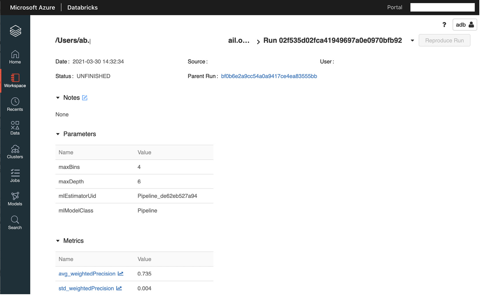
图 10.2 – MLflow 模型注册表 UI

我们可以通过在搜索运行框中传递一个参数来显式查找这些运行的具体结果。例如，我们可以通过传递 maxDepth 超参数中使用 6 的值时得到的结果="literal">params.maxDepth = 6 在搜索框中。

我们还可以通过创建用于特定性能指标的超参数的不同值的散点图来比较结果，这在我们尝试查找和比较最佳超参数集。

下一节将深入探讨一种更自动的方法，以找到最小化某个函数的最佳超参数集。我们将使用损失函数来做到这一点。我们将使用 Hyperopt 来定义和探索搜索空间，并找到最小化损失函数的超参数。

Azure Databricks Runtime for Machine Learning 包括 Hyperopt，这是一个 Python 库，旨在用于分布式计算系统，以促进一组最优超参数的学习过程。它的核心是一个库，它接收我们需要最小化或最大化的函数，以及一组定义搜索空间的参数。有了这些信息，Hyperopt 将探索搜索空间以找到最佳的超参数集。 Hyperopt 使用随机搜索算法来探索搜索空间，这比使用传统的确定性方法（如随机搜索或网格搜索）要高效得多。

Hyperopt 针对在分布式计算环境中的使用进行了优化，并提供了对诸如 PySpark MLlib 和 Horovord 等库的支持，后者是用于分布式深度学习的库 我们稍后将重点介绍的培训。它也可以应用于单机环境以及其他更常见的库，例如 TensorFlow 和 PyTorch。

使用 Hyperopt 时的一般工作流程如下：

1. First, we must find the function that we want to optimize. This can be either a performance metric that we want to maximize or a loss function that we want to minimize.
2. Next, we must define the conditional search space in which Hyperopt will scan for the best parameters to optimize the defined target function. Hyperopt supports several algorithms being used in the same run, which allows us to define more than one model to explore.
3. After that, we must define the search algorithm that will be used to scan the search space.
4. Finally, we can start the exploration process by running the fmin() Hyperopt function. This will take the objective function as an argument and the search space for identifying the optimal set of parameters.

话虽如此，Hyperopt 最关键的两个部分如下：

• The objective function that we will pass as the optimization target. Generally, this is a loss function or a performance metric.
• A dictionary of hyperparameters that define the search space. We can choose different distributions for each set of hyperparameter values.

在下一部分中，我们将学习如何将 Hyperopt 应用到 Azure Databricks Runtime for Machine Learning，以找到特定任务的最佳超参数，而不管应用的算法如何。

Hyperopt concepts

在本节中，我们将通过 Hyperopt 的某些概念来确定其核心功能，以及我们如何使用它们来有效地扫描搜索空间以查找有助于最小化或最大化我们的目标函数。正如我们之前提到的，当我们开始使用 Hyperopt 时，我们必须定义以下内容：

• The objective function
• The search space that we will scan
• The database that will be used to save the result of evaluating the points in the search space
• The search algorithm that will be used to scan the search space

在这里，我们的主要目标是找到代表最佳超参数的最佳标量集。 Hyperopt 允许我们详细定义搜索空间，以提供有关目标函数在搜索空间中的哪个位置执行得更好的信息。其他优化库通常假设搜索空间是具有相同分布的较大向量空间的子集，但通常情况并非如此。 Hyperopt 让我们定义搜索空间的方式使我们能够执行更有效的扫描。

Hyperopt 允许我们非常简单地定义目标函数，但是当我们增加参数数量时，它也会增加复杂性，我们希望在执行过程中跟踪。最简单的例子如下，我们找到x的值，它使一个线性函数最小化，y(x) = x ：

from hyperopt import fmin, tpe, hp
best_param = fmin(
    fn=lambda x: x,
    space=hp.uniform('x', 0, 1),
    algo=tpe.suggest,
    max_evals=100)
print(best_param)

我们可以通过分解参数来分解之前的执行：

• The Hyperopt fmin() function takes in the fn keyword argument and the function to minimize. In this case, we are using a very simple lambda function; that is, f(y)=x.
• The space argument is used to pass the search space. Here, we are using the hp function from Hyperopt to specify a uniform search space for the x variable in the range of 0 to 1. hp.uniform is a function that's built into the library that helps us specify the search space for specific variables.
• The algo parameter is used to select the search algorithm. In this case, tpe stands for Parzen estimators. We can also set these parameters to hyperopt.random.suggest. The search algorithm is an entire subject, so we will only briefly mention this, but you are free to search for more details about the types of algorithms that Hyperopt applies to find the most suitable set of hyperparameters for you.
• Lastly, the maximum number of evaluations is specified using the max_evals parameters.

一旦我们指定了所有必需的参数，我们就可以开始运行，它将返回一个 Python 字典，其中包含最小化目标函数的指定变量的值。

尽管我们这里的最小工作示例看起来非常简单，但 Hyperopt 的复杂性随着我们在优化目标函数时所拥有的规范数量而增加。当我们提出最佳策略时，我们可以问自己的一些问题如下：

• What type of information is required besides the actual returned value of the fmin() function? We can obtain statistics and other data that is collected during the process and might be useful for us to keep.
• Is it necessary for us to use an optimization algorithm that requires more than one input value?
• Should we parallelize this process and if so, do we want communication between these parallel processes?

回答这些问题将定义我们实施优化策略的方式。

在并行优化过程中，Hyperopt优化算法与目标函数之间发生通信，以获得目标函数在搜索空间特定点的实际值。在这种通信中，在该浮点损失中返回目标函数的值（也称为负效用）与搜索空间中的该点相关联。

此处显示的简单示例说明了使用 Hyperopt 定义目标函数和搜索空间是多么简单。但是，在我们想要存储更多信息而不仅仅是搜索空间中目标函数返回的浮点值的情况下，它仍然存在不足。它也是一种不与搜索算法或并发函数交互的评估。

为了解决第一个问题，我们可以使用一个目标函数，该函数通过返回一个嵌套字典来检索多个值，其中包含所需的统计和诊断的键值。为此，我们有一组强制值，我们的目标函数必须返回：

• status: We can choose one of the keys from hyperopt.STATUS_STRINGS to show the status of competition. This way, we can track if our evaluation was completed successfully or if it failed.
• loss: This is the float value that is returned by the actual objective function when it is evaluated in that specific point in the search space. It must be present if the status of the competition is OK.

我们还可以在目标函数的选项中指定 一些额外的可选参数。这些关键值如下：

• loss_variance: A float value specifying the certainty of the stochastic objective function.
• true_loss: You can store the loss of the model with this name so that we can use the built-in plotting tool. This is especially useful when we are working with hyperparameter optimization because it allows us to plot the results of the exploration very simply.
• true_loss_variance: The uncertainty of the loss of the model.

此功能允许我们将这些值存储在与 JSON 兼容的数据库中，例如 MongoDB。下面的代码示例向我们展示了如何定义一个非常简单的 f(x) = x 目标函数，它将执行状态作为键值字典返回：

import pickle
import time
from hyperopt import fmin, tpe, hp, STATUS_OK
def objective(x):
    return {'loss': x, 'status': STATUS_OK }
best = fmin(objective,
    space=hp.uniform('x', -5, 5),
    algo=tpe.suggest,
    max_evals=50)
print(best)

我们可以通过使用 Trials 对象充分利用能够返回字典的优势，这允许我们在执行优化时存储更多信息。在以下示例中，我们正在修改目标函数以返回更复杂的输出，该输出稍后将存储在 Trials 对象中。我们可以通过将其 作为 Hyperopt fmin() 函数的参数传递来做到这一点：

import pickle
import time
from hyperopt import fmin, tpe, hp, STATUS_OK, Trials
def objective(x):
    return {
        'loss': x,
        'status': STATUS_OK,
        'eval_time': time.time(),
        'more_data': {'type': None, 'value': [0, 1]},
        'attachments':
            {'time_module': pickle.dumps(time.time)}
        }
trials_obj = Trials()
best_params = fmin(objective,
    space=hp.uniform('x', -5, 5),
    algo=tpe.suggest,
    max_evals=50,
    trials=trials_obj)
print(best_params)

执行完成后，我们可以访问 Trials 对象来检查目标函数在优化期间返回的值。我们有不同的方式可以访问存储在 Trials 对象中的值：

• trials.trials: Returns a list of dictionaries with all the parameters of the search.
• trials.results: The dictionaries that are returned by the objective function.
• trials.losses(): The actual losses of all the successful trials.
• trials.statuses(): The status of each of the trials.

这个Trials对象可以保存为pickle对象或者使用自定义代码解析，让我们对结果有更深入的了解审判。

可以像这样访问试验的附件：

msg = trials.trial_attachments(trials.trials[0])['time_module']
time_module = pickle.loads(msg)

在此示例中，我们正在获取第一次试用的 time_module 附件。

需要注意的重要一点是，在 Azure Databricks 中，我们可以选择将 Trials 和 SparkTrials 对象传递给fmin() 函数的试验参数。当我们执行单机算法（例如 scikit-learn 模型）作为目标函数时，会传递 SparkTrials 对象。在这里，Trials 对象用于分布式训练算法，例如 MLlib 或 Horovod 模型。 SparkTrials 类允许我们分发优化的执行，而无需引入任何自定义逻辑。它还改进了计算分配给工作人员。

不要将 SparkTrials 对象与为分布式训练设计的算法一起使用，因为这将导致在集群中并行执行。

现在我们对如何配置 fmin() Hyperopt 函数的基本参数有了更清晰的了解，我们可以深入了解如何定义搜索空间。

Defining a search space

我们可以将 搜索空间表示为一组嵌套函数，这些函数 为不同的测试用例定义了单独的搜索空间。例如，在下面的代码块中，我们为 x 参数指定搜索空间，其中包含两个名为 test_space_1 的测试空间和test_space_2:

from hyperopt import hp
search_space = hp.choice('a',
    [('test_space_1', 1 + hp.lognormal('x', 0, 1)),
     ('test_space_2', hp.uniform('y', -5, 5))
    ])

在这里，Hyperopt 将根据搜索算法从这些嵌套的随机表达式中进行采样。该算法采用自适应探索策略，而不仅仅是从搜索空间中抽取样本。在前面的示例中，我们定义了三个参数：

• a: Selects the case to be used
• test_space_1: Generates positive values for the x parameter
• test_space_2: Generates positive values for the y parameter

每个表达式都有标签作为第一个参数，算法在内部使用该标签将参数选择返回给调用者。在此示例中，代码的工作方式如下：

• If the a variable is 0, we will use x and not y.
• If the a variable is 1, then y will be used but not x.

x 和 y 变量是条件参数，取决于 a 的值的结果 。如果我们以这种条件方式对变量进行编码，则说明 x 变量在 a 时对目标函数没有影响为 0，这有助于搜索算法以更有效的方式分配信用。这利用了用户对要分析的目标函数的领域知识。

search_space 是一个变量空间，它被定义为一个图形表达式，描述了如何在不生成搜索空间的情况下对一个点进行采样。这优化了执行的内存和计算使用。这些图表达式称为 pyll 图，并在 hyperopt.pyll > 类。

您可以通过采样来探索示例搜索空间：

import hyperopt.pyll.stochastic
print(hyperopt.pyll.stochastic.sample(search_space))

我们现在知道如何定义优化目标函数的搜索空间。重要的是要注意，我们定义要在搜索空间中测试的案例的方式也会影响搜索算法在自适应搜索期间对试验的工作方式。在下一部分中，我们将了解在 Azure Databricks 中使用 Hyperopt 的一些最佳做法。

Applying best practices in Hyperopt

到目前为止，我们已经讨论了如何指定要最小化的目标函数的执行以及我们将在其中评估它的搜索空间。此外，我们已经看到有在我们如何定义探索超参数的可能值的方式以及如何通过在搜索空间中定义条件参数来利用领域知识方面具有很大的灵活性。

我们必须牢记 Hyperopt 库本身的某些方面，以及它在 Azure Databricks 中的执行方式。以下是在 Azure Databricks 中使用 Hyperopt 优化目标函数时需要记住的一些重要概念：

• The Hyperopt Tree of Partzen Estimator algorithm is a Bayesian method that's much more efficient than common grid and random search approaches. It allows us to scan a larger set of possible hyperparameters. Apply the domain knowledge when defining the search space to improve the performance of the exploration.
• When we use hyperopt.choice() and MLflow to track the progress of the optimization, Mlflow will log the index of the choice list. We can fetch the parameter values using the Hyperopt hyperopt.space_eval() function.
• When working on large datasets, it is always advisable to experiment on small subsets of the data to incrementally learn about the optimal search space. This helps us define the one that will be used on the entire dataset.
• When we use the SparkTrials object, it is advisable to use CPU-only clusters. This is because in Azure Databricks, parallelism is reduced in the GPU clusters in comparison to the CPU ones.
• Do not use SparkTrials on autoscaling clusters as the parallelism value is selected at the beginning of the execution. Therefore, if the cluster scales, it won't improve the performance of the execution.

应用这些概念将确保我们利用 Azure Databricks 中的 Hyperopt 优化执行。在下一节中，我们将详细了解如何在 Azure Databricks 中改进深度学习模型的推理。

正如我们在前面的章节中看到的 ，Hyperopt 是一个 Python 库，它允许我们跟踪优化 可用于超参数模型调优分布式计算环境< /a> 例如 Azure Databricks。在本节中，我们将通过一个训练 scikit-learn 模型的示例。我们将使用 Hyperopt 跟踪调优过程并将结果记录到模型生命周期管理平台 MLflow。

在用于机器学习的 Azure Databricks Runtime 中，我们可以使用 Hyperopt 的优化版本，它支持 MLflow 跟踪。在这里，我们可以使用 SparkTrials 对象来记录并行执行期间单机模型的调优过程的结果。我们将使用这些工具为几个 scikit-learn 模型找到最佳的超参数集。

我们将执行以下操作：

• Prepare the training dataset.
• Use Hyperopt to define the objective function to be minimized.
• Define an Hyperopt search space, over which we will scan for the best hyperparameters.
• Define the search algorithm that will be used to scan the search space.
• Execute the optimization and track the best set of parameters in MLflow.

让我们开始吧：

1. First, we will import all the necessary libraries that we will be using:

   import numpy as np
   from sklearn.datasets import fetch_california_housing
   from sklearn.model_selection import cross_val_score
   from sklearn.svm import SVC
   from sklearn.ensemble import RandomForestClassifier
   from sklearn.linear_model import LogisticRegression
   from hyperopt import fmin, tpe, hp, SparkTrials, STATUS_OK, Trials
   import mlflow

   Copy
2. In this example, we will be using the California housing dataset, which is included as an example dataset in scikit-learn. This dataset holds data from the 1990 US census with house values for 20,000 houses in California, along with some features with data about income, number of inhabitants, rooms, and so on. To fetch this dataset, we will use the fetch_california_housing() scikit-learn function and dump the results into variables named features and target:

   features, target = fetch_california_housing(return_X_y=True)

   Copy
3. Now that we have split our dataset into the features and the target, we will scale the prediction variables, which is a common practice in machine learning and deep learning. This way, we will ensure we have scaling consistency. This will help us overcome several problems that arise when our features have not been discretized into scaled variables. The features that are available in our dataset are as follows:

   a) 每块房屋收入中位数

   b) 房屋年龄

   c) 每栋房屋的平均房间数

   d) 平均卧室数量

   e) 总区块人口

   f) 平均住户人数

   g) 纬度

   h) 经度

4. By reviewing the scale of the features in each column – a simple operation that can be done in a pandas DataFrame using the describe() method – we can see that the orders of magnitude in the mean values vary a lot:

   import pandas as pd
   features_df = pd.DataFrame(features)
   features_df.describe()

   Copy
5. As we can see, the ranges and scales of these variables can be very different:
   

   图 10.3 – 特征的统计总结

6. The population of a block is measured in thousands, but the average number of bedrooms is centered around 1.1. To prevent situations in which features with large values are deemed to be more important, scaling the features and normalizing them is a standard practice. To normalize the features so that they're the same scale, we can use the scikit-learn StandardScaler function:

   from sklearn.preprocessing import StandardScaler
   scaler = StandardScaler()
   scaled_features = scaler.fit_transform(features)

   Copy
7. Now that we have scaled the predictor features, we can check that the mean is close to 0 by calling the mean(axis=0) NumPy method on the scaled_features dataset:

   scaled_features.mean(axis=0)

   Copy
8. Now that our predictor features have been normalized and scaled, we will have to convert the numeric target column into discrete values:
   

   图 10.4 – 缩放特征意味着

9. This target column vector is the value of each house and is a continuous positive scalar. We will transform this into a target column vector with discrete values that are 1 when the house value is greater than the mean and 0 where it is not. This way, the prediction can be framed as a question; for example, given the predictor features, is the values of this house greater than the mean? To discretize the values, we will compare this with the mean and use the numpy.where() function to convert the Booleans values that the comparison yields into 1s and 0s:

   target_discrete = np.where(target < np.median(target), 0, 1)

   Copy

   这样，我们将目标变量编码为具有两个级别（1 或 0）的列向量。这表明房价是否高于均值。

10. Now that we have prepared our dataset, we can start setting the stage for optimizing the hyperparameters of several scikit-learn models that we will use to train an effective classification model. To this end, we will use the following three scikit-learn classifier models:

    a) 支持向量机

    b) 逻辑回归

    c) 随机森林

11. We will create an objective function to be minimized that will be passed to Hyperopt. This will run the training and calculate the cross-validation performance metric over several types of models, defined as 'type' parameters. One thing to bear in mind about this function is that because we are using the fmin() Hyperopt function, this will try to minimize the objective function. So, to improve the performance metric – which is accuracy, in this case – we must use the negative accuracy. Otherwise, Hyperopt will try to minimize the accuracy, which is something that we obviously don't want to do:

    def objective(params):
        classifier_type = params['type']
        del params['type']
        if classifier_type == 'svm':
            clf = SVC(**params)
        elif classifier_type == 'rf':
            clf = RandomForestClassifier(**params)
        elif classifier_type == 'logreg':
            clf = LogisticRegression(**params)
        else:
            return 0
        accuracy = cross_val_score(
                                   clf, 
                                   scaled_features, 
                                   target_discrete).mean()
        return {'loss': -accuracy, 'status': STATUS_OK}

    Copy

    请注意，此函数的输出是具有两个必需参数的键值字典。它们是“损失”（负精度）和“状态”（使用我们之前导入的 Hyperopt 状态字符串之一定义）。

12. The next step is to define the search space we will use to scan all the possible hyperparameters for each of the selected scikit-learn models. This will help us find the one that yields the best accuracy. We will use the hyperopt.choice() function to select the different models and specify the search space for each classification algorithm. The label of this selection is classifier_type. It will iterate over the previously defined types of algorithms in the objective function based on the given labels in the search space:

    search_space = hp.choice('classifier_type', [
        {
            'type': 'svm',
            'C': hp.lognormal('SVM_C', 0, 1.0),
            'kernel': hp.choice('kernel', ['linear', 'rbf'])
        },
        {
            'type': 'rf',
            'max_depth': hp.quniform('max_depth', 1, 3, 5),
            'criterion': hp.choice('criterion', ['gini', 'entropy'])
        },
        {
            'type': 'logreg',
            'C': hp.lognormal('LR_C', 0, 1.0),
            'solver': hp.choice('solver', ['liblinear', 'lbfgs'])
        },
    ])

    Copy

    搜索空间表达式内的 hyperopt.choice() 函数将传递 'type' 参数 到目标函数，该函数又创建一个名为内部变量"literal">classifier_type 并使用 它来选择 适当的算法。然后它将剩余的参数传递给模型。请注意，在目标函数中，'type' 参数是如何在创建内部变量后被删除的，以避免目标算法中任何可能的命名冲突。

13. Now, we must choose the search algorithm that will be used to scan the search space. As we have seen previously, Hyperopt provides us with two main options for this:

    a) hyperopt.tpe.suggest：这是 Parzen 估计器树 (TPE) 算法，这是一种贝叶斯算法，根据之前的结果自适应地选择超参数。

    b) hyperopt.rand.suggest：这是一种随机搜索算法，与 TPE 算法的不同之处在于它是一个 non -在搜索空间上使用采样策略的自适应方法。

14. In this example, we will use the TPE algorithm, so we will choose tpe.suggest, as shown here:

    search_algorithm = tpe.suggest

    Copy
15. The next step is to define the object that will hold the results of each of the trials. We will use SparkTrials to keep track of the progress of the exploration and log it in MLflow. As we mentioned previously, we will use the SparkTrials object instead of the native Trials Hyperopt object because we are using algorithms designed to be run on a single machine. If we were to use an MLlib algorithm, we must use the MLflow API to keep track of the Trials result.

    反过来，SparkTrials 是 一个可以接收两个 可选参数的对象，如 如下：

    a) parallelism：这是并行拟合和评估的算法数量。此参数的默认值等于可用的 Spark 任务槽数。

    b) timeout：fmin() 可以运行的最长时间（以秒为单位）。没有最长时间限制。

    Spark 中默认的 parallelism 值为 8。建议的设置是将此值显式设置为正值，因为 Spark 任务槽取决于集群的大小。

16. The final step of preparing the optimization run is to use the mlflow.start_run() MLflow wrapper. We will use it to log the results of this exploration in the MLflow platform. This will automatically keep track of the progress of the run, along with all the defined variables and labels in the objective function and search space:

    with mlflow.start_run():
      best_hyperparams = fmin(
        fn=objective, 
        space=search_space,
        algo=search_algorithm,
        max_evals=32,
        trials= SparkTrials())

    Copy
17. The max_evals parameter allows us to specify the maximum number of points in the search space that will be evaluated. So, we can consider this value to be the maximum number of models that Hyperopt will fit and evaluate for each search space:
    

    图 10.5 – 使用 MLflow 跟踪训练运行

18. Once the execution has been finalized, we can examine the hyperparameters that produced the best result:

    import hyperopt
    print(hyperopt.space_eval(search_space,
                              best_hyperparams))

    Copy

    我们应该看到 最佳超参数集 在控制台中打印为“键值字典”以及名称和在定义的最小化函数的搜索空间中找到的最佳参数值：

    

图 10.6 – 最佳超参数

我们可以点击experiment图标查看MLflow实验笔记本的右上角。此 选项将显示在运行和，正如我们之前提到的，允许我们可视化产生最佳结果的一组超参数和算法。我们还可以检查改变特定参数的效果。

通过这种方式，我们可以同时调整多个模型，并跟踪模型在每个定义的搜索空间中的性能。借助 Hyperopt 和 MLflow，我们可以轻松定义高级管道，以使用 Azure Databricks Runtime for Machine Learning 并行微调模型。

在本章中，我们了解了 Azure Databricks 的一些有价值的功能，这些功能使我们能够使用 MLflow 模型注册表跟踪训练运行，以及找到机器学习模型的最佳超参数集。我们还学习了如何优化使用 Hyperopt 扫描最优参数的搜索空间。这是一组很棒的工具，因为我们可以微调对用于训练的超参数具有完整跟踪的模型。我们还使用自适应搜索策略探索了定义的超参数搜索空间，该策略比常见的网格和随机搜索策略优化得多。

在下一章中，我们将探讨如何使用集成到 Azure Databricks 中的 MLflow 模型注册表。 MLflow 可以更轻松地跟踪机器学习模型的整个生命周期以及训练过程中使用的所有相关参数和工件，但它也允许我们轻松部署这些模型，以便我们可以发出 REST API 请求以获取预测。 Azure Databricks 中的这种 MLflow 集成增强了创建和部署机器学习模型的整个工作流程。